How databases fit in
This is the first (draft) chapter of a new book on relational databases (using Postgres) that I’m working on as a summer project. Stay tuned for additional chapters. The book under development can also be viewed at Leanpub, which supports commenting, and also will allow me to bundle the book with video lectures. I appreciate your feedback!
Introduction #
Imagine that you work in a small direct-response mail order company that takes orders from customers by phone. Each agent in the call center downstairs has a stack of paper order forms on his desk, and when he receives an order he writes down the product name(s), quantity ordered, and the customer’s address and payment information. He uses a calculator or computer to sum up the order total, and tells the customer how much they’ll be charged.
Periodically, a data entry worker visits the call center and picks up stacks of filled-in order forms. She enters each order’s details into a file on her desktop computer, perhaps a big Excel spreadsheet that she’s designed herself for this task. At the end of the day, when all the orders are entered, she sends the complete file to two other departments: fulfillment, which processes the customer’s credit card and packs and ships the orders, and accounting, which calculates each salesperson’s commission.
This is the kind of process that a small business might develop when it’s first getting started, and in fact, it’s exactly the process that I encountered when I was first learning about databases at a small company in Maine. Unfortunately, simple processes like this tend to get complicated as the company gets bigger, and can become impossible to maintain. Just a few of the challenges this company might face are:
When the business grows to the point that multiple data entry workers are needed, they must coordinate their work somehow. Perhaps each worker creates her own file, and they must combine them at the end of the day. There are many opportunities for errors to enter the system.
If a payment is declined, or if a customer returns an order, one of the old spreadsheets must be updated, but which one? The data is kept in the order it was entered, not alphabetized by customer, and if there are now multiple spreadsheets for each day of business, searching for the old order is a big challenge.
As a result of the update made by fulfillment or customer service, multiple versions of the data exist. Accounting still has the old data, and they need to be notified of the change so they can correct the salesperson’s commission. Even if they’re sent the modified file, how do they know which row(s) are changed? And as more changes are made over time, who is responsible for keeping the official record?
As the business grows, the order entry data may change. For example, product numbers or names may change, discounts or coupon codes may be introduced, or some kind of membership number may be offered to frequent customers. As the paper order forms change, the spreadsheets must also be modified. Consequently, today’s data files look different from last month’s and even more different from last year’s. As people change jobs and leave the company, can their replacements even read the older data?
As this small business becomes a medium-sized enterprise, the seeming convenience of using a spreadsheet can become a nightmare of data management. Before long, the data entry workers, accountants, and other departments may find they spend more time managing spreadsheets than doing their main jobs. And sooner or later, management may wish to use the historical order data for a new purpose, such as customer relationship management (CRM) or business intelligence (BI). What they’ll find is that the data is spread out over a huge number of files, with multiple versions of each file existing in different places, and older files having a different structure and meaning from newer files. What a mess!
Aside: There are lots of other problems we could imagine in this scenario, but I wanted to keep it brief. One that ought to be mentioned is the security disaster posed by this system. The spreadsheet in my story contains customers’ credit card numbers as well as personally identifying information, and it’s being passed around willy-nilly between departments. Moreover, any employee with a grievance could walk out the door with all of the data on a thumb drive, and who would know?
A database #
Imagine instead if there was a black box in the office into which all those order forms were fed. At any time, a person could ask the black box to retrieve any order record (or list of records) by time and date, by customer name, by product, or another attribute. Fulfillment could ask for the payments waiting to be processed, and it would get a printout of exactly that. Shipping could request invoices and mailing labels for orders ready to ship. Accounting could ask for the sum of order totals taken by each salesperson for a given time period. Moreover, changes could be filed in the black box and all subsequent requests would include the up-to-date, corrected information. The black box serves as the manager of, and the official system of record for, all the company’s order data.
That’s the big idea of a database. Instead of having every person or department or program keep its own copy of the data, a database serves as a system of record, a “single source of truth” that can always be accessed by everyone who needs it for their different purposes. A database stores some knowledge about the data’s structure and meaning, or metadata, so diverse users can know what they’re looking at. And most importantly, a database offers flexible but easy-to-use query methods so that users can request just the data they want, whether it’s a single record, a collection of data, or an aggregation into averages, counts, or sums.
A variety of databases #
Databases come in many shapes and sizes and they serve a lot of different purposes. Most often, a database acts as a server, that is, a software program that is always on, waiting for requests and responding to them. It’s necessary for databases to always be on and available if people and other software systems are going to depend on them to store data. (Otherwise, those people and programs will have to store their own data locally, which defeats the purpose of a database – independent and shared data management.)
A database administrator (DBA) is therefore responsible for a key component of a business’s IT infrastructure. If the database goes down, a lot of other programs go down, so the DBA ought to learn best practices for managing security, keeping backups and recovering from disasters. Maintaining and upgrading a database has been compared to maintaining a sailing ship when it is out to sea. The DBA can’t just take the database out of service to work on it however he wants; the business must stay afloat.
Server-based databases vary widely in scale and scope. Some databases support a single application, such as a dynamic website, and these may run on the same physical computer as the application’s code. A larger database might run on a dedicated machine that multiple users access over the network; for example, a company may keep a database of customer relationship information which can be accessed by sales, marketing, and customer service systems.
Aside: The term “server” means a software or hardware system that is constantly listening for requests or commands and reacting to them. When a software server runs on a computer dedicated to that purpose, the computer itself is also called a “server”.
Larger still are enterprise-scale databases that integrate a wide variety of subject areas. This category includes enterprise resource planning (ERP) systems that integrate several areas of business operations, and enterprise data warehouses (EDW) used for analysis and reporting of business performance. Enterprise-scale databases may run on mainframes or may be distributed over large clusters of dozens or hundreds of computers.
Aside: It is worth noting that there are also what we may call “personal” or “desktop” databases that run on personal computers and do not remain active when not in use. These databases are created with programs such as SQLite and Microsoft Access (the two you’re most likely to encounter) and are saved as files. They have many of the features for structuring and querying data that you’ll learn from this book, such as the SQL query language, but for business use they would still pose most of the same problems as the spreadsheets in my opening vignette. You would still end up with lots of different versions of the same (database) files with inconsistent data kept by different people and departments.
If your goal is simply to learn SQL or relational data modeling, though, SQLite and Access are both fine choices.
What you’ll learn from this book #
This book will introduce you to relational databases, with data modeling and SQL first and foremost. It covers the scope of a typical first database course in an information systems or analytics program at the university level. It can be used as a textbook for an instructor-led course—instructors, please contact the author for an instructor’s guide, slides and materials–or used for self-guided study with or without the video lectures produced by the author (coming soon via Leanpub).
My main goal in creating this book is to make data modeling and SQL understandable to the reader, so it may serve as a good low-cost supplement for students who are struggling with a theory-heavy textbook and having a hard time getting the point. Instead of starting with loads of theory up-front, I’ll take a more pragmatic approach based on relational data modeling “patterns” and examples.
This book will also provide a lot of practice using SQL, the structured query language common to all relational databases, because the most frequent feedback I’ve heard from my students at Arizona State (and from companies that hire them) is that they need more practice with SQL.
The database of choice for this book is PostgreSQL (often nicknamed “Postgres”), an open-source database that has become quite popular with developers in recent years. Compared to some other popular databases like SQL Server and MySQL, there aren’t many good books about Postgres, so I hope this book will be valuable if only for its examples. Postgres makes a good choice for teaching because it is free software (both “free as in free speech” and “free as in free beer”), and because it runs on all the major platforms—Windows, Mac OS, and Linux—so you can follow this book no matter what kind of computer you have handy.
Rest assured that the lessons of this book are transferable to other relational databases. Each of the major brands has its own quirks and special features, but this book mainly covers the fundamentals that apply everywhere. As currently planned, one chapter will exhibit some of PostgreSQL’s special features.
Aside: If this book finds any significant success with readers, I fully intend to create additional versions of the text that highlight SQLite, MySQL, Access, or whatever other platforms people are interested in. Give me feedback!
Lab 1: your first PostgreSQL database #
Up and running with Postgres #
PostgreSQL is available for free at www.postgresql.org and is extremely well documented there. Installation instructions will vary depending on your platform, and should be pretty straightforward. You can probably accept all the default configuration options. Be sure to remember the password you set during installation. You’re up and running when you can enter the command psql -V at your system’s command line, and the system responds by telling you the version of PostgreSQL installed. At the time of this writing, it looks like this for me:
$ psql -V
psql (PostgreSQL) 9.5.3
If that doesn’t make any sense to you, see Appendix A for my detailed guide to installing Postgres on Windows, Mac, and Linux, or refer to the online documentation.
Relations are tables #
Databases can be classified according to the types of abstractions they allow you to model your data with. In a relational database, data is modeled as a set of tables with structured rows and columns. Other data models are possible. In a document-oriented database such as MongoDB, data is modeled as documents with tree-like structures. In a graph database like Neo4J, data is structured as a network diagram (a mathematical graph) with nodes and edges. Compared to those newer forms, the relational model is far more commonly seen and better understood, and is the most versatile. Relational databases have been tried and tested in business for nearly four decades, and are probably the best tool for the job in all but a few specialized cases.
The tables you find in a relational database are properly called relations. A relation is not just any table; it is a construct found in set theory and is defined by the following characteristics:
- Every row has the same columns.
- Column names must all be different.
- Each column is defined to contain just one specific type of data.
- Each row must be unique; usually we enforce this by adding a machine-generated ID number to each row. This column is known as the “primary key” column.
- No inherent ordering of rows or columns, or other information about how to display the data, is stored in the table.
Consequently, a relation is a simpler and less flexible structure than a table you might create in a spreadsheet program like Microsoft Excel. Spreadsheets allow you to mix data types, to have rows with different numbers of columns, and to decorate your data with display logic like fonts, colors, and sizing. Figures 1-1 and 1-2 illustrate the comparison with an example of sales data that might be recorded by a small outdoor sports mail-order business.
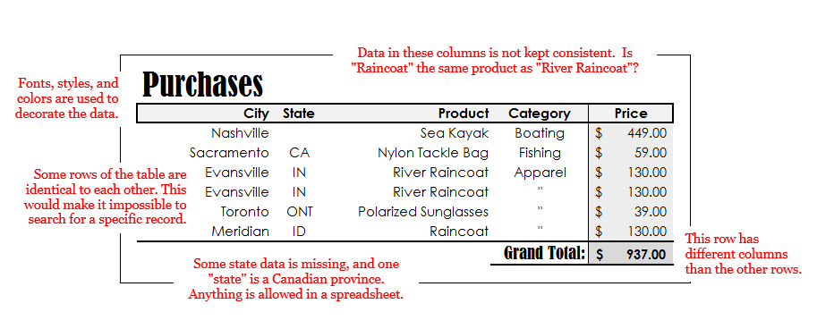
In a spreadsheet the user can be lax in data entry, for example omitting the state “TN” when we all know where Nashville is, or entering a quotation mark (meaning “ditto”) instead of spelling something out. Data types unanticipated at the time the table was designed could be inserted freely; for example, a three-letter Canadian province abbreviation could be inserted into a column meant for two-letter US states. Although these are convenient for data entry, they may lead to problems for computer systems that want to use the data (for example, to print mailing labels). The spreadsheet user can also decorate the data with fonts, styles, sizes and colors in order to make it more readable, and he can add extra information like a “grand total” row.
As seen in Figure 1-2, a database table (or relation) is much more strictly defined. Data types must be specified in advance for each column, guaranteeing uniformity. That means special cases must be anticipated before they occur. In this example, the database designer specified that state abbreviations must be exactly two characters, and that the price may be numeric (allowing fractions) rather than integer. In order to guarantee that each row is unique, and therefore can be looked up, the databsae users has added a primary key column and populate it with an auto-generated ID number.
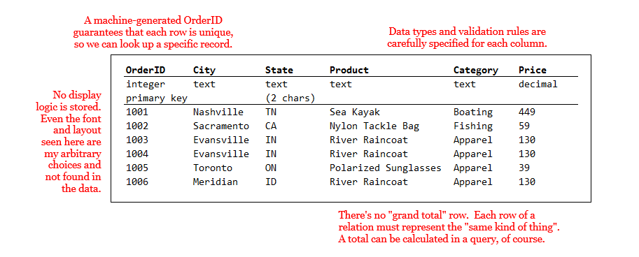
No other information is found in the rows of a relation except the data itself: not fonts and styles, and not even the sort order. Totals, averages, and the like wouldn’t be stored in the table either, because rows correspond only to individual data “records”. Aggregated values like totals and averages could be calculated in a query or perhaps stored in additional tables created specifically for the purpose.
Creating your first relation #
Let’s fire up PostgreSQL and create a table. (I probably won’t use the word “relation” much after this, except for a bit of theory in Chapter 2. Where I write “table”, you should be able to figure out what I mean.)
First, a note about the term “database”. As I have described it above, a database is a system that organizes and stores data and, importantly, makes it available to people who need to search or retrieve it. Others more precise than I will distinguish between the database, which is the organized data store, and the database management system (DBMS) which is a program like PostgreSQL that creates the database and grants access to it. When we call PostgreSQL (or Oracle, or SQL Server, etc.) a database, we are using the term more generally to include both the database and the DBMS, since they go together.
To understand how we interact with PostgreSQL, though, you need a third definition of the term. In PostgreSQL, a database is a logical subdivision of the data store, which in some other systems might be called a tablespace. You may create any number of tables grouped into databases on the same server. (For the purposes of this book’s labs, your personal computer is acting as a PostgreSQL server.) Table names must be unique within a database, but not within a server. If several examples in this book include a table called “customers”, you can avoid a conflict by creating a new database for each lab.
What we’ll do in this first lab, then, is:
- Create a PostgreSQL database called “lab1”
- Log in to that database with
psql - Create a table of Purchases
- Query the single-table database with SQL
Database creation #
You can create a database from your operating system’s command line (i.e., before logging in to PostgreSQL with psql or another front-end tool), by using the command createdb. The basic structure of this command is createdb [OPTIONS] [DBNAME], and you can learn more by typing createdb --help at the command prompt. The only optional parameter you need to specify is the identity of the database “user” that was created when you installed PostgreSQL. The user “postgres” is the superuser who has power to make any and all changes to the server, including creating databases. Thus, the following command creates a database called “lab1”:
$ createdb -U postgres lab1
If you did not specify a username with the -U parameter, createdb tries to log in to PostgreSQL with your computer account’s username (in my case, “Joseph”). If I have set up such an account, createdb lab1 would work. But since I haven’t, it fails. One of the Challenges offered at the end of this chapter is to find out how to create a user account to make these commands less verbose.
If necessary, you can also drop (i.e., delete) the new database from the commmand line, with:
$ dropdb -U postgres lab1
For future reference, you can alse create and delete databases using SQL once you’re logged in to psql: the CREATE DATABASE and DROP DATABASE commands, respectively. One way or another, create that database, which will be home to your first table.
Introducing psql #
The command-line client for PostgreSQL is psql, and like createdb, it needs to know the username you want to connect with. Connect with psql -U postgres. This will not open a new window, but rather you will see a brief welcome and the command prompt will be different from the operating system’s default prompt.
$ psql -U postgres
psql (9.5.3)
Type "help" for help.

postgres=#
The change in the command prompt means you’re in a different environment. Here, you can enter SQL queries or some commands specific to psql. The first thing I’d recommend you do is type help, which introduces you to a few of the latter. Most psql commands begin with a backslash (\) and you can get a full listing of them by entering the command \?. If you need to quit, \q is the command for that. If you want to, take some time now to explore the lists of SQL queries and psql commands possible.
postgres=# help
You are using psql, the command-line interface to PostgreSQL.
Type:  \copyright for distribution terms
       \h for help with SQL commands
       \? for help with psql commands
       \g or terminate with semicolon to execute query
       \q to quit
By default, when you start psql you’re connecting to the default database, which like the superuser is called “postgres”. Any SQL commands you enter at the prompt will be executed on that database’s tables, which isn’t what you want. To switch over to the new database you created, use the \c command:
postgres=# \c lab1
You are now connected to database "lab1" as user "postgres".
lab1=#
Notice that the prompt changes to tell you which database you’re working in.
Creating a table #
To create a table in the “lab1” database, we use the aptly-named SQL CREATE TABLE command. I will expand on its usage in Chapter 2, but the basic form of it is as follows:
CREATE TABLE table_name (
   column_name    data_type   [OPTIONS],
   ...
   );
As I mentioned, one of the special characteristics of a relation is that each column allows data only of a specified type. PostgreSQL offers a number of built-in data types, such as numeric, text, date, and more. I will discuss the choice of data type more in Chapters 2 and 8, but it need not delay an introductory example. There are many optional clauses available in the CREATE TABLE statement which can be discussed later or looked up in the documentation; the only one we need now is PRIMARY KEY, a flag which indicates that a particular column is going to contain unique values that may be used to look up specific rows later.
The command to create our table of Purchases is as follows. You may type this in at the psql prompt, even if it spans several lines. The code won’t execute until the semicolon (;) is reached. Mind the cases: in PostgreSQL the SQL keywords (i.e. CREATE TABLE, PRIMARY KEY, and the data types) may be uppercase or lowercase, but you should only use lower case letters and underscores (_) for the table and column names. PostgreSQL isn’t very sensitive to whitespace, so you can enter this code all on one line, or spread out over several lines, with indentation and tabs if you want them.
CREATE TABLE purchases (
order_id integer PRIMARY KEY,
city text,
state char(2),
product text,
category text,
price numeric );
If the command succeeded, you’ll see “CREATE TABLE” in the output. If there’s an error message instead, don’t worry, just try again. The most likely causes of errors are typos in the data types, the wrong number of commas, and uppercase letters in the table or column names. If the command worked but you defined the table incorrectly, the easiest solution is to start over by issuing the command DROP TABLE purchases; and creating the table anew.
You can confirm that the table exists with the psql command \dt, which displays a table of all the tables in the currently selected database:
lab1=# \dt
           List of relations
 Schema |   Name    | Type  |  Owner
---------------------------------------
 public | purchases | table | postgres
 (1 row)
That’s all there is to defining a table, at least an empty one. In order for us to demonstrate some SQL queries, though, we’ll need to store some data in the table with the SQL INSERT command. We’ll use the simplest form of this command, adding only one row at a time to the table, for example:
INSERT INTO purchases VALUES
(1001, 'Nashville', 'TN', 'Sea Kayak', 'Boating', 449);
Take note that text data must be wrapped in quotation marks ('), and numbers must not.
Writing INSERT commands by hand will quickly become tiresome, and is not the usual mode of entering data into a real database. Typically the database will support software (such as a web app, or an enterprise system) that generates data insertion and update commands automatically. Another way we might load a lot of data quickly is to read in a file containing (presumably machine-generated) INSERT commands. In psql you can execute SQL commands from a file using the \i command.
I have provided a script file containing 100 lines of purchase data on the GitHub repository that supports this book. You may find the file purchases.txt at https://github.com/joeclark-phd/databasebook-postgres, in the “psql_scripts” folder. I have downloaded this file to my computer, a Windows laptop, and saved it in the directory C:/psql_scripts, so for me the command looks like this:
lab1=# \i c:/psql_scripts/purchases.sql
INSERT 0 1
...
Be sure to use the correct file path for your operating system and the location where you downloaded the script.
Regardless of how you insert data into the table, please add at least several records so that you can try some meaningful queries in the next section. If you are experiencing errors with INSERT commands, check that the number of values you’re inserting matches the number of columns in the table, that they’re in the right order, and that the order_id number is unique for each inserted row. If you run into problems, you can empty the table by entering the command DELETE FROM purchases; and start again.
Querying your data with SQL #
SQL is the structured query language more or less common to all relational databases, and it really shines for its ability to extract just the data you want from a table or group of tables. What kinds of queries might you want to make of this data? You might want specific subsets of the data, such as all the orders for a particular product or in a particular state. Or you might want to aggregate the data, that is, sum or count or average them, perhaps in groups. Even with one simple table, there are quite a few ways to query it.
Let’s start with the basics. Your first query is the simplest: it just requests all the data.
SELECT * FROM purchases;
That’s quite a lot of rows, so I’ll give you a trick to shorten the results. Affix “LIMIT ” to the end of the query to get only the first several rows:
SELECT * FROM purchases
LIMIT 10;
The meaning of the “*” is “all columns”. It’s possible to request only certain columns, for example, let’s say you only want to know the cities and states that your customers are ordering from. Specify the desired columns in the “SELECT” clause:
SELECT city, state
FROM purchases
LIMIT 10;
Most of the time you don’t want every row, but want to select a subset of the data. This is accomplished with the “WHERE” clause of a query. You may request a single row by its primary key, for example:
SELECT *
FROM purchases
WHERE order_id = 1011;
Or you may give criteria that qualify more than one row, if you want to see a specific subset. For example:
SELECT *
FROM purchases
WHERE state='ME';
The criteria don’t have to be “equality” conditions, by the way. We can also use numerical inequalities; any row for which the inequality is “true” will be returned:
SELECT city, state, product
FROM purchases
WHERE price > 500;
Another condition you might use, for a primitive text search, is “LIKE”. The “%” character is a wildcard that matches any text. Thus, the following code returns all data where the product name ends in “Kayak” but would not return data where there was additional text after that word.
SELECT city, state, product
FROM purchases
WHERE product LIKE '%Kayak';
Aggregate queries #
The queries above allow you to carve out subsets of the data by requesting only certain columns, certain rows, or both. In every example, though, the rows you get in the result are rows from the original table. Aggregate queries are those that generate data by combining the original rows via an aggregation function, usually SUM, COUNT, or AVERAGE. Obviously the sum of two rows is one row, and is not identical to either of the original rows. The following query gives you the total dollar amount of all purchases in the table:
SELECT SUM(price)
FROM purchases;
No matter how many rows were in the original table, the query above returns just one row. Say… how many rows are in the original table?
SELECT COUNT(order_id)
FROM purchases;
The COUNT function actually counts the number of rows, not the number of unique values. If you used COUNT(state) instead of COUNT(order_id) you’d get the same result. Even if you have five hundred purchases in 50 states, the COUNT would be 500, not 50. Since the parameter given to the COUNT function doesn’t matter, it’s often easier to simply use COUNT(*).
A grand total (or count, or average) is interesting, but a lot of the time what we want to do are compare subtotals (or counts, or averages) for various groupings of the data. To do this, we introduce a “GROUP BY” clause. If we want to know how many purchases were made in each of several categories, we can group by the “category” column and count up the rows in each group:
SELECT category, COUNT(*)
FROM purchases
GROUP BY category;
If you want to know which products account for the largest portions of your revenue, you might group by product and sum the order prices. There are a lot of products, though, so it’s helpful to sort the results with an “ORDER BY” clause. Since the sum is the 2nd column of the result data, that’ll be “ORDER BY 2”.
SELECT product, SUM(price)
FROM purchases
GROUP BY product
ORDER BY 2;
To get just the top ten, here’s a trick: sort the data in descending (“DESC”) order, and “LIMIT” the results to just the first ten rows.
SELECT product, SUM(price)
FROM purchases
GROUP BY product
ORDER BY 2 DESC
LIMIT 10;
In Chapter 3 and beyond you’ll learn a lot more SQL, such as how to create queries that “join” multiple tables, and how to write queries that employ nested sub-queries. Even in this example, though, you’ve seen several of the main parts of a SELECT query, including the “WHERE”, “GROUP BY”, and “ORDER BY” clauses, and aggregate queries. You have begun to see that even a simple one-table database may be queried in several different ways, and that doing this with short SQL queries may be much easier than trying to wrangle the data in Excel.
I recommend that you attempt the exercises and challenges at the end of this chapter to get more practice with the basics of relational databases, SQL, and PostgreSQL specifically.
Read more at Leanpub.