The relational model
This is the second (draft) chapter of a new book on relational databases (using Postgres) that I’m working on as a side project. Stay tuned for additional chapters. The book under development can also be viewed at Leanpub, which supports commenting, and also will allow me to bundle the book with video lectures. I appreciate your feedback!
There are other data models #
For a couple of decades (roughly 1985-2005), the relational data model was the only game in town, you had to learn it, and there was no reason for a textbook to argue the point. Today, data engineers have a lot of other options. Document-oriented databases are booming in popularity with app developers for their ease of use; graph databases have captured the imagination of researchers and tinkerers because of their natural fit with social network applications; and the analytics world has found performance advantages to be gained with dimensional databases, column-family databases, and cluster-based Big Data platforms like Hadoop. These are meaningful advantages, so before we take it for granted that the relational model is the most important one to learn, it is necessary to remind ourselves what it is and what its unique advantages are.
A data model is a means of describing the data in a database without regard to the way it is actually physically stored. It provides abstractions that humans can work with—e.g. tables, documents, dimensions—instead of implementation artifacts like bytes, pointers, and disk sectors. This abstraction is quite important when you consider the growth and evolution of a database over time, and the number of applications that might come to depend on it. As databases are used, they grow larger, the types of data stored may grow or change, and it may be necessary for database administrators to optimize their performance by upgrading the technology in various ways. If the developers of applications that depend on these databases had written their code to interact with the data as it was stored on disk, their applications would break, and code would need to be rewritten, every time such a change was made. But because we have data models, this is not necessary. Application developers interact with the database using a “data language” that is independent of physical implementation; they query tables, rows, and columns for instance, instead of locations on disk.
The relational model’s particular strength is its ability to efficiently answer queries that were not foreseen at the time the database was developed. Before E.F. Codd’s landmark paper introducing the relational model, the leading approach to data modeling was a hierarchy or network in which you would follow links from one data point to another. Consider, for example, a hierarchical database of movies listed by director:
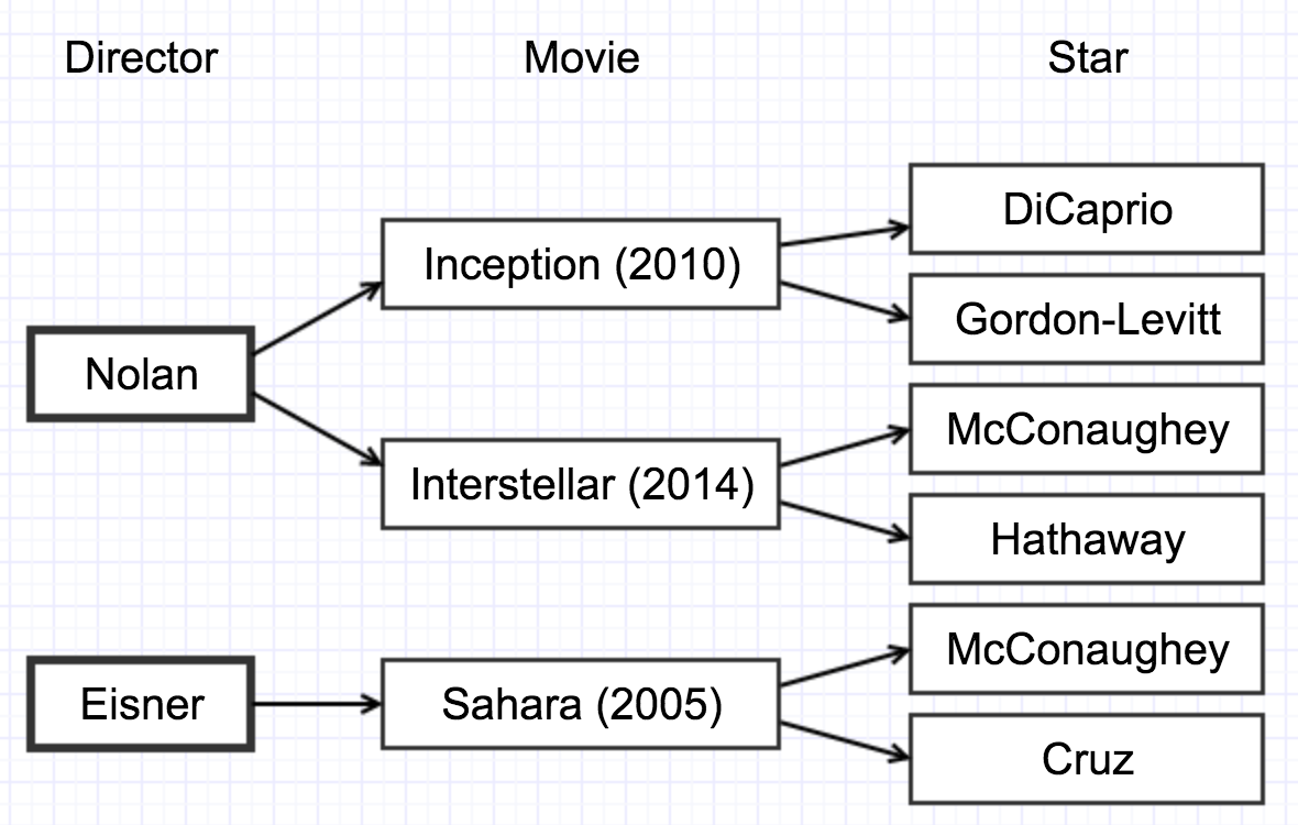
[Figure 2-1. hierarchical database of movies]
In this example, it would be very easy to query the database for a list of movies directed by Christopher Nolan; just start from his name and follow the pointers. By contrast, it would be quite difficult (computationally) to query for a list of movies in which Matthew McConaughey had appeared. The database engine would have to essentially read through the entire database, the vast majority of which is not relevant to the query, following all paths from left to right in the diagram to make sure it had found all of the paths that end with his name. In a really huge database, such a query could be prohibitively expensive.
The problem is, as databases grow, you will always find that you want to make queries you didn’t anticipate at the time you created the database. Codd, a researcher at IBM, had this problem in mind when in a 1970 he published “A Relational Model of Data Storage”.

[Figure 2-2. Edgar F. Codd]
In the relational model, the database consists of a set of tables, one for each entity (or noun) described by data. Each table can be queried on its own, or related tables can be combined into one query, but there is no “parent” table and no network or hierarchy that must be traversed. You have already seen a glimpse of this in Chapter 1; now, let’s define the terms a bit more precisely.
Theoretical roots #
Codd’s conception of a relation comes from set theory:
The term relation is used here in its accepted mathematical sense. Given sets S1, S2, …, Sn (not necessarily distinct), R is a relation on these n sets if it is a set of n-tuples each of which has its first element from S1, its second element from S2, and so on. We shall refer to Sj as the j th domain of R.
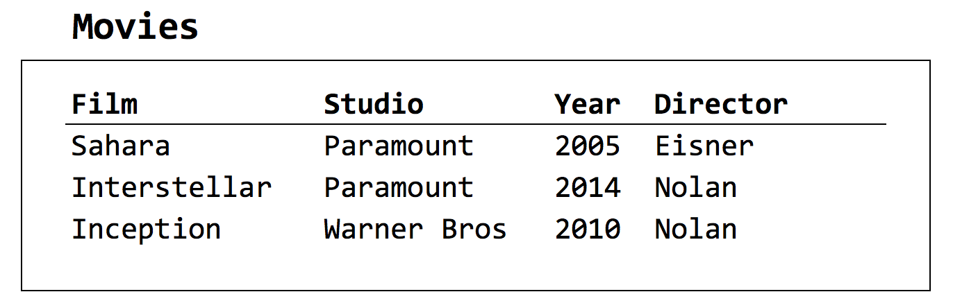
It is possible to visualize this as a table, hence the commonly-used language of tables, rows, and columns. In Figure 2.3, we see a relation defined by four sets—a set of movie titles, a set of movie studios, the set of integer years, and the set of director names. These indicate the possible values that may appear in any given data record; it’s not necessarily the case that all of the years of history (for example) will be found in the data. This is an important point: the relation (table) is “defined” by specifying the domains (columns) and not by the rows. You’ll see this in SQL’s CREATE TABLE command, which specifies column names and data types only.
[Figure 2-3. A relation with four domains, three tuples]
The term tuple (derived from “double”, “triple”, “quadruple”, and so on, up to “n-tuple”) in mathematics refers to an ordered list of values. In this context, a tuple fits in to a relation if it contains one value for each domain, in the same ordering as the domains. So in the above example, a tuple must contain a movie title, a studio name, an integer, and a director’s name, in that order. Each such tuple is a “row” of the table, or a record of the data—in this case, it’s a movie that we’re interested in.
Because a relation is a set of tuples so defined, a number of constraints apply—some of which will be relaxed in practical implementations. These include:
- Each row must be unique.
- The order of rows is immaterial.
- The order of columns is significant.
- Each row must include a value for each column.
The first rule is easy to accidentally violate, for example in an order-taking system, where the same customer may purchase the same product on more than one occasion. It is common practice therefore to add a primary key (PK) column that contains a value guaranteed to be unique in the relation, such as an identification number.
The second rule implies that we must query the database without regard to the order in which data was entered, or any other order. One cannot query for the “next” value and reliably predict what result will be given. Attention must be paid to the WHERE clause of a SQL query to specify exactly what we want.
In practice, the third rule is ignored. Codd informs us that the mathematical term for a relation with no specific domain ordering is a relationship. Instead of referencing an element of a row by its position in the sequence, in practice we use column names. Database developers should give sensible names to their columns, particularly when there may be one or more with the same domain of potential values. For example, a table of customer records may have two or more “address” columns, one for billing and one for shipping. It would be wise to give these columns names that indicate both the domain and the role, such as “billing_address” and “shipping_address”.
The fourth rule may be relaxed as well. Allowing missing values (called nulls) in certain columns gives database developers the flexibility to include optional attributes, or to add a data record in a step-by-step way instead of all at once. Obviously nulls cannot be allowed in every column, or the first rule may be violated. Therefore most databases don’t allow nulls in the primary key column.
In a query result, which otherwise resembles a relation, even the first two rules may be violated. This can be demonstrated by the following database interaction:
ch2=# select studio from movies;
 year
---------
 Paramount
 Paramount
 Warner Bros
(3 rows)

ch2=# select movie, year from movies order by year;
 movie         | year
---------------+------
 Sahara        | 2005
 Inception     | 2010
 Interstellar  | 2014
(3 rows)
The first result contains non-unique rows. There’s a mathematical term for a set of n-tuples that admits duplicates: it’s called a bag. The second example result orders the rows in a meaningful sequence.
A relational database is a database of relations #
We can therefore think about a relational database as a collection of tables (technically relations (even more technically, relationships)) that, together, describe the important facts in whatever context we’re interested in: a business, an application, a research project, or whatever. In some cases, a table may be useful on its own, but in many tasks you will want to query two or more related tables together. Yes, tables are related: customers are assigned to salespeople, employees belong to departments, products have bills of materials that go into their manufacture.
Two aspects of the context must be represented in the database design: entities and relationships. Entities are the nouns that matter: people, things, places, events, and concepts. Relationships are connections between entities which can usually be described by verbs. The most useful tool in developing a data model is an entity-relationship diagram (aka E-R diagram or ERD). See Figure 2-4. The boxes are entity types (although we usually just say “entities”), which correspond to tables. The lines indicate the relationship types (or “relationships”), which indicate how the rows of each table relate to the rows of the other tables.
ASIDE: Relationships, not relations; Also, this use of “relationships” differs from the mathematical term introduced above.
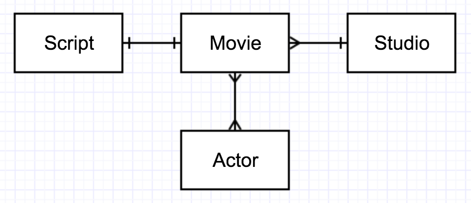
[figure 2-4. a sample ERD with 1:1, 1:M, and M:M relationships]
Three types (cardinalities) of relationships are depicted in Figure 2-4, a relational data model for a database of movies (like IMDB) diagrammed in “crow’s foot” notation. These are a “one-to-many” (or 1:M) relationship between Studio and Movie, a “one-to-one” (1:1) relationship between Script and Movie, and a “many-to-many” (M:M) relationship between Movie and Actor. Out of these three basic cardinality cases, complex data models can be designed.
ASIDE: You’ll see me use the term “relational model” in a couple of different ways. On the one hand, when we talk about “-the- relational model”, we mean the set of principles for designing relational databases, as contrasted with e.g. -the- dimensional model or -the- graph model. On the other hand, I may talk about “-a- relational model” for a database; this is a specific set of tables designed for a particular scenario, also known as a **schema. Figure 2-4 depicts a schema for a movie database.
ASIDE: There are a few other notations for E-R diagrams, and which one you use is a matter of personal preference. (Unless you’re in my database class; in that case, use the crow’s foot notation.) I use an online program called Gliffy to draw the diagrams.
One-to-many #
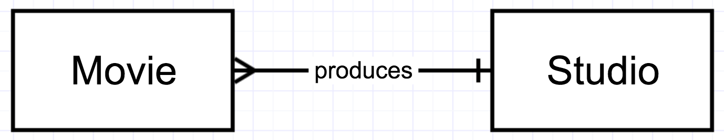
The most common type of relationship between tables is one-to-many (1:M), as seen in Figure 2-5. The rectangles in the diagram stand for entity types, which correspond to tables, and mean that any number of entity instances of each type may be in the database. We can assume that there are, or will eventually be, a large number of movies in the Movie table and large number of studios in the Studio table. The line with a crow’s foot at one end and a single tick mark at the other end indicates the type of relationship that may exist between rows of the Movie table and rows of the Studio table. Simply put, it says that each movie is related to just one studio, but that any given studio may be related to more than one movie. It is also common practice to add text to the diagram to explain why, or how, the two entity types might be related—in this case, studios produce movies (and movies are produced by studios).
[Figure 2-5. A one-to-many relationship]
ASIDE: A very common mistake I see in my classes is that students draw boxes on diagrams for specific -instances- of entity types. It would be wrong to, for example, have a rectangle on this diagram for the movie Interstellar or the studio Paramount. Those instances will become rows, but in an E-R diagram we are concerned with the tables.
When it comes time to create the actual tables, a one-to-many relationship is implemented by a simple and intuitive mechanism called a foreign key (FK). Remember that each table has a primary key, a column of data whose values are guaranteed to be unique—typically an ID number or code. To implement a 1:M relationship we add a special column to the table on the “many” side (in Figure 2-5, “Movie”) that holds references to primary key values in the other table. This could be achieved with the following SQL (note the REFERENCES clause):
CREATE TABLE studio (
 id  integer  PRIMARY KEY,
 name text );

CREATE TABLE movie (
 id  integer  PRIMARY KEY,
 title text,
 studio_id integer REFERENCES studio(id) );
If we view the tables with a few sample rows of data (Figure 2-6), the purpose of the foreign key column studio_id should be clear. At a glance you can see that Sahara and Interstellar were produced by Paramount (studio #1) and that Inception was produced by Warner Bros. (studio #2).
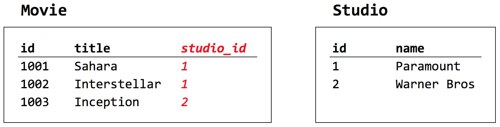
[Figure 2-6. Sample tables in a 1:M relationship (emphasis on foreign key column)]
Notice that there is no foreign key in the “Studio” table. If you pencil in a “movie_id” column on Figure 2-6, or simply imagine one, the reason should be obvious. If a studio were assigned a “movie_id”, then a studio could only be related to one movie, and that clearly doesn’t mesh with reality or with our E-R diagram.
Many-to-many #
The next most common kind of relationshp between two entity types is many-to-many (M:M), as in the relationship between Movies and Actors: each movie involves more than one actor, and each actor can be in more than one movie. See figure 2-7.
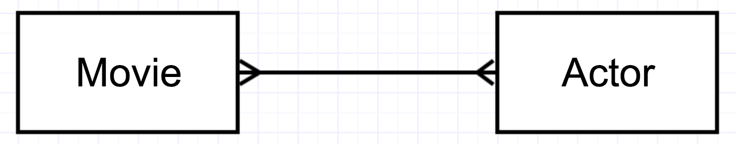
[Figure 2-7. A many-to-many relationship]
Now, an M:M relationship is easy to draw on a diagram, but it’s a little more complicated to implement as real tables in the database. Take a minute to think about how you might do it, before reading about it below.
…
Did you come up with a solution?
Well, here’s the solution that I teach my students: to represent the many-to-many connection, you need a third table. This is the only kind of case where a table represents a relationship rather than an entity. This new table, called an associative relation, might have two columns only: each a foreign key to one of the tables in the relationship. Figure 2-8 illustrates some sample data for the simplest kind of associative table.
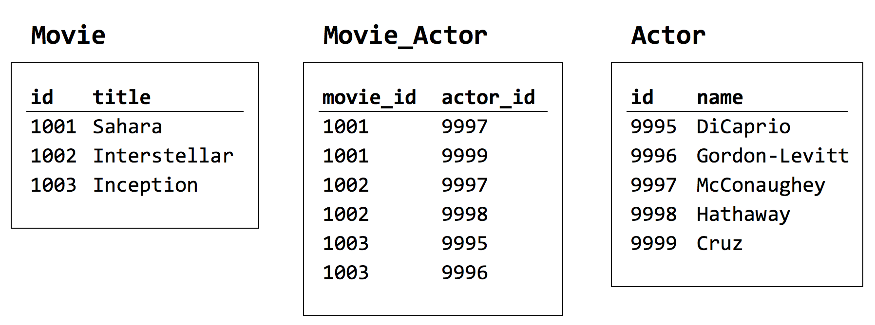
[Figure 2-8. Movie_Actor creates the relationship between Movie and Actor]
A question of style concerns whether you should depict the associative entity on your E-R diagram—essentially as a table with two 1:M relationships to the entities of interest—or simply use the double-crow’s-foot notation as in Figure 2-7.
To answer this, consider the opportunity afforded by the existence of an associative table. It need not be limited to two foreign key columns only, because a table can have any number of columns. You can therefore use columns of the associative table to give meaningful characteristics about the relationship. Such a relationship may in fact be a “thing” of its own, perhaps an intangible one. An M:M relationship between a Buyer and a Seller might be an entity called a Contract. An M:M relationship between a social media User and a channel he follows could be called a Subscription. And in the case of the Actor-Movie relationship, we might call it a Role.
The answer to the style question is that, if the associative table can be construed as an associative entity, a thing or concept (or noun) meaningful to the business, it makes sense to add it to the diagram. If the associative entity is meaningless to anyone except the guy writing database code, you would in most cases leave it off the diagram.
See Figure 2-9 for an example diagram including the associative entity. Note that instead of an M:M relationship you now see two 1:M relationships. In this example, the rectangles representing entities also show the names of some columns that would belong to each table; this is also a common style of E-R diagramming.
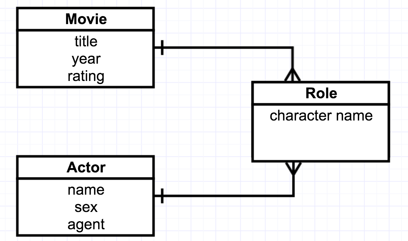
[Figure 2-9. Many-to-many relationship with meaningful associative entity.]
An implementation in SQL could look like this:
CREATE TABLE movie (
 id integer PRIMARY KEY,
 title text,
 year integer );

CREATE TABLE actor (
 id integer PRIMARY KEY,
 name text );

CREATE TABLE role (
 id integer PRIMARY KEY,
 movie_id integer REFERENCES movie(id),
 actor_id integer REFERENCES actor(id),
 character_name text );
Notice that there are two foreign keys in the role table.
One-to-one #
One-to-one (1:1) relationships are much less common than 1:M and M:M relationships, simply because if two types of entities are related this way it’s often easier to put them together in one table. For example, a person has only one Social Security number, and a Social Security number has only one person, so you would typically have a table for People and include a Social Security number column rather than having two tables.
One reason you might store the data in separate tables is if some of the data needs to be stored in a different (physical) space, or stored with different security settings. Physical database optimization is beyond the scope of this chapter (although we’ll come back to it in Chapter 8) but I’ll give you and example. In many web applications, each user has a profile picture. Picture files (JPEG, PNG, or whatever) are quite large on disk, and to include them in the Users table of the database would make that table larger (perhaps by orders of magnitude) hence making queries slower. To give your website users a quicker response time, you might store the pictures in a separate ProfilePicture table, and relate them by foreign key to the corresponding rows of the Users table.
Another use case for a 1:1 relationship is when one of the tables contains “optional” data. For example, let’s say our movie database contains 10,000 rows, and we have scripts for 1,000 of those movies. Rather than have a script column in the Movie table, with 9,000 NULL entries making that table bigger and slower, we could have a separate Script table with only the rows it needs. In this case, each row of Script relates to exactly one row of Movie, but each row of Movie may relate to zero or one row of Script. It’s not exactly a parnership among equals: Movie is the main table in the relationship, and Script is a “dependent”.
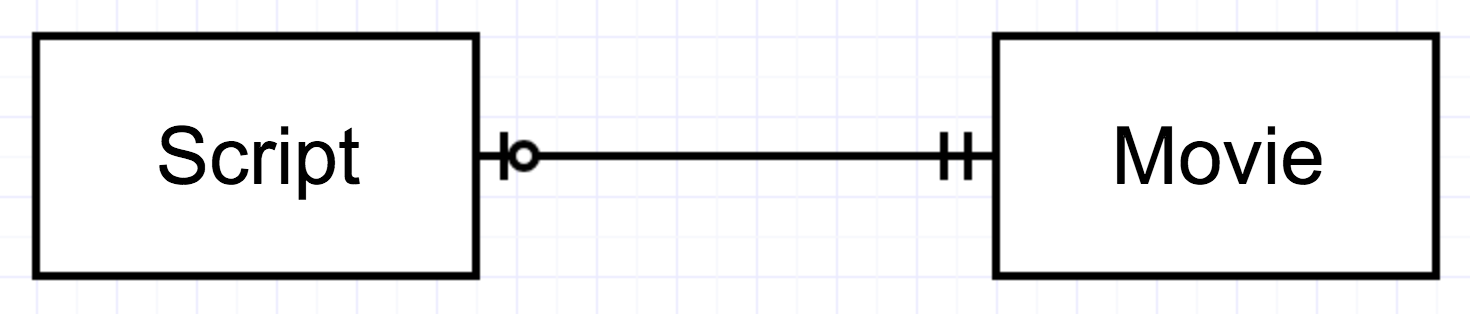
[Figure 2-10. One-to-one relationship between Script (optional) and Movie (required)]
Figure 2-10 uses a version of the crow’s foot notation that indicates the difference. The double tick mark next to Movie means that, for any row of Script, there must be at least one and no more than one row of Movie. The circle (or zero) with a tick mark next to Script means that for any row of Movie, there may be zero or one rows of Script. (The simpler notation was seen earlier, in Figure 2-4.)
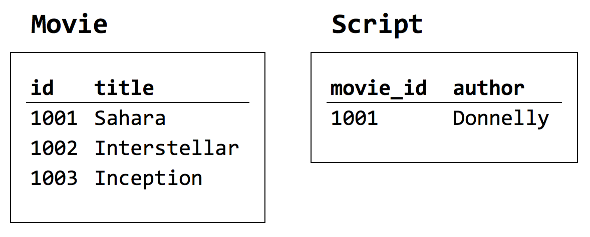
To implement this in SQL, even though you could get away with putting the foreign key on either side of this relationship, or on both, the best practice is to put a foreign key in the “dependent” table. In this case, that table is Script. Essentially a 1:1 relationship is a special case of 1:M, where the foreign key is simply constrained to be unique. Since primary keys are unique, the most practical way to do this is for the rows of the dependent table to have the same primary key values found in the “independent” table, and for its primary key to double as a foreign key, like so:
CREATE TABLE movie (
 id integer PRIMARY KEY,
 title text,
 year integer );

CREATE TABLE script (
 movie_id integer PRIMARY KEY REFERENCES movie(id),
 author text,
 body text );
A selection of the data, as in Figure 2-11, shows that the Script table borrows its primary key values from Movie but does not have a row for every value.
[Figure 2-11. Sample data from tables in a 1:1 relationship]
Unary relationships #
All of the relationships in the E-R diagrams seen so far have been binary relationships, meaning they include two tables, and are said to have degree of two. Other degrees are possible. Frequently we also see unary relationships, where rows of one table are related to other rows of the same table. Unary relationships can be of any cardinality we’ve seen so far: 1:M, M:M, or 1:1. Remember that it is not the tables that are related, per se, but the rows.
An example of a unary 1:M relationship is posed by Figure 2-12, which depicts a movie studio ownership relationship. Studios are often owned by other studios, as for example Disney owns Lucasfilm and Sony owns Columbia. This can be expressed as a foreign key in the Studio table referencing an “owner”. (Note that it can’t be done with a foreign key referencing the “owned” studio; the FK belongs on the “dependent” side of a 1:M relationship.)

[Figure 2-12. A unary 1:M relationship]
Here it is in SQL. The NULL keyword indicates that owner is an optional field; it may contain NULL if a particular studio has no owner recorded in our database.
CREATE TABLE studio (
 id  integer  PRIMARY KEY,
 name text,
 owner integer NULL REFERENCES studio(id) );
As in other cases, sample data may be helpful to illustrate how the implementation works.

[Figure 2-13. Sample data for a unary 1:M relationship]
A unary many-to-many relationship could easily represent ties of affiliation between individuals or organizations. Hollywood being the way it is, we could define a M:M relationship between Actors called “was married to”. Like binary M:M relationships, this would require an associative table (which may or may not be diagrammed). See Figure 2-14.
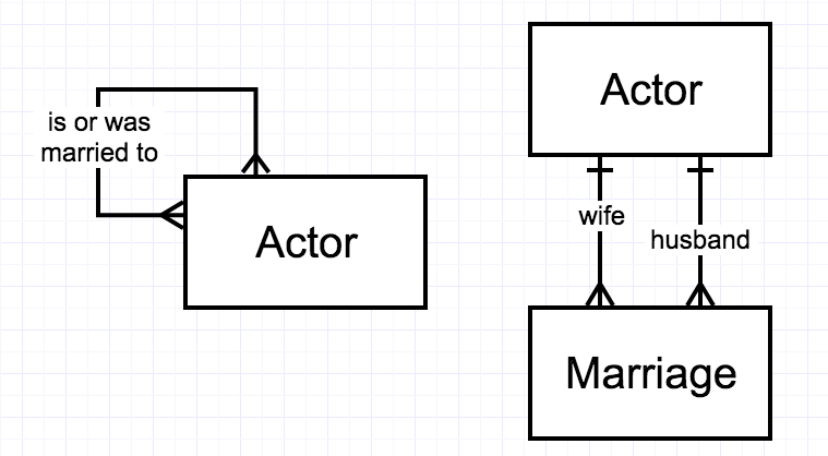
[Figure 2-14. Two ways to diagram Hollywood marriages as a unary M:M relationship.]
An implementation in SQL could look like this:
CREATE TABLE actor (
 id integer PRIMARY KEY,
 name text );

CREATE TABLE marriage (
 id integer PRIMARY KEY,
 husband integer REFERENCES actor(id),
 wife integer REFERENCES actor(id) );
And some sample data illustrates how it works:
ch2=# select * from actor;
  id  |        name
------+--------------------
 9001 | Brad Pitt
 9002 | Angelina Jolie
 9003 | Jennifer Aniston
 9004 | Billy Bob Thornton
(4 rows)

ch2=# select * from marriage;
 id | husband | wife
----+---------+------
  1 |    9001 | 9003
  2 |    9004 | 9002
  3 |    9001 | 9002
(3 rows)
Finally, an example of a unary 1:1 relationship that might be found in our movie database as a reference from a sequel to its predecessor. This would be implemented as an optional column in the Movie table called “sequel_to”, referencing another row of the Movie table, like so:
ch2=# select * from movie;
 id |   title   | sequel_to
----+-----------+-----------
  1 | Rocky     |
  2 | Rocky II  |         1
  3 | Rocky III |         2
  4 | Rocky IV  |         3
  5 | Rocky V   |         4
(5 rows)
Ternary and n-ary relationships #
Virtually all of the relationships you’ll find in most E-R diagrams are binary (connecting two tables) or unary (connecting rows within one table). It is nevertheless possible, however uncommon, to imagine a relationship connecting three tables (“ternary”), four (“quarternary”), or any arbitrary number of tables (“n-ary”). This simply means that one of each entity type is required to create a case of the relationship.
In the context of movies, we might consider a distribution deal to be one such relationship. A movie distribution deal is an agreement between a producer (Studio) and a third party (Distributor) to distribute a movie (Movie) in a particular territory (Territory). Figure 2-15 illustrates this as a quarternary many-to-many-to-many-to-many (M:M:M:M) relationship.
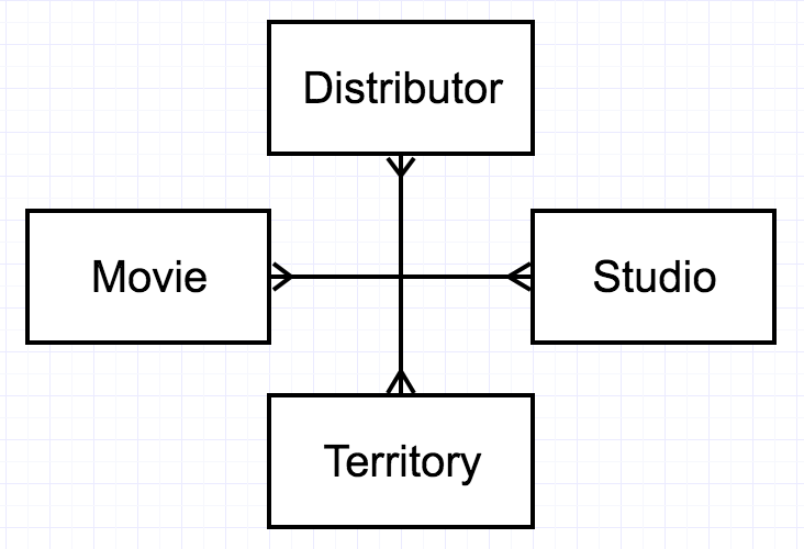
[Figure 2-15. An example of a quarternary M:M:M:M relationship.]
It is rare to see this kind of relationship diagrammed, though. The only way to implement a relationship of degree > 2 is to use an associative table with foreign key columns for all the participants. Therefore, in most cases you will simply model a new associative entity—for example “Deal” or “Contract”—which contains details as well as 1:M relationships with each of the related tables.
Summary #
The relational data model is one of several data modeling paradigms used by databases today, albeit the most popular one. At the heart of the relational model is a construct called a relation, which we typically call a “table”, although it has some strict constraints such that not any table will qualify. The particular strength of the relational model is that it enables database users to efficiently execute queries that were not anticipated at the time the database was designed. This flexibility is obtained by breaking down the data into numerous tables, one for each “entity” or meaningful noun concept in the domain, and by relating these tables to each other by means of foreign key columns. The relationships that may be defined differ in cardinality and degree. Cardinality refers to how many rows of each table participate in a relationship, and the possibilities are one-to-many (1:M), many-to-many (M:M), and one-to-one (1:1). Degree refers to how many tables are related. Binary (two table) and unary (one table) relationships are the most common ones you will encounter. A relational database model can be visualized as an entity-relationship (E-R) diagram, and you are encouraged to become familiar with at least one E-R diagram notation, such as the “crow’s foot” notation summarized in Figure 2-16.
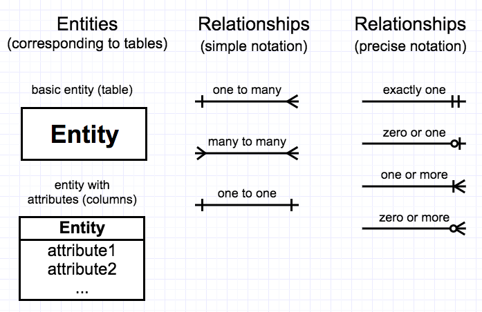
[Figure 2-16. Symbols in the crow’s foot notation for E-R diagrams]
Lab 2: Creating and querying a relational database #
In Lab 1 you created a one-table database and were introduced to some of the basic things you can do with SQL queries. Now that you have learned the basics of how multiple tables can be related to one another within a relational database, you will want to see some richer and more realistic examples. Moreover, you’ll need to familiarize yourself with the main way that tables are queried together: the SQL join.
What we’ll do in this lab is:
- Create a new database called “lab2”.
- Define several tables to learn the features of the CREATE TABLE command.
- Learn how to code different types of JOIN queries
In order to get started, first create a new empty Postgres database called “lab2”, log in to your Postgres server using psql, and switch your context to the new database—much as we did in Lab 1:
$ createdb lab2
$ psql
psql (9.6.1)
Type "help" for help.

joeclark=# \c lab2
You are now connected to database "lab2" as user "joeclark".
lab2=#
The CREATE TABLE command #
SQL is divided into two main types of commands, called data definition language (DDL) and data manipulation language (DML) respectively. DDL commands are those used to design and structure the tables that constitute the database, and the chief among them is CREATE TABLE. (Two others you may frequently encounter are ALTER TABLE and DROP TABLE.) The basic form of a CREATE TABLE command in Postgres is as follows:
CREATE TABLE table_name (
  column_name data_type [constraints/options],
  column_name data_type [constraints/options],
  ...,
  [constraints]
);
I’ve kept it simple here in order to make a clear introduction, and will reveal more options as we move on. The complete specification of CREATE TABLE can be found in the PostgreSQL online documentation, which is excellent. You have already seen several examples of CREATE TABLE, one of which I’ll reproduce here:
CREATE TABLE studio (
  studio_id integer PRIMARY KEY,
  name text
);
ASIDE: Postgres makes things easier if the names of your tables and columns are lowercase and contain no special symbols other than underscores and digits. If you want to use uppercase letters or spaces in these identifiers, it’s possible, but you must always remember to surround them with doublequotes, e.g., CREATE TABLE "Movie Studio". Different database systems have different naming conventions. See the documentation for details.
In this example you saw only one of PostgreSQL’s optional constraints: PRIMARY KEY. Yes, a “PK” is a constraint on the data. By that we mean that it sets up a rule that will lead to errors if we try to insert bad data—here’s one of the advantages of databases as opposed to spreadsheets: they tell us when we make mistakes. In this case, the rule is the entity integrity rule, which dictates that the primary key column must contain a unique (not null) value for every row. Look what happens if I try to add two movie studios with the same “studio_id”:
lab2=# insert into studio (studio_id,name) values (1,'Disney');
INSERT 0 1
lab2=# insert into studio (studio_id,name) values (1,'Warner Bros');
ERROR:  duplicate key value violates unique constraint "studio_pkey"
DETAIL:  Key (studio_id)=(1) already exists.
Three other constraints you’ll see me use in this lab are NOT NULL, which means a particular column can’t be empty, REFERENCES which sets up a foreign key relationship, and CHECK which allows for arbitrary validation of the data.
Developing your database iteratively #
As you work through this and other labs, you’ll soon find that you’ve made mistakes or come up with better ideas, and want to start over. Typing those CREATE TABLE commands into psql gets tedious and is error-prone. As in most other types of programming, the solution is to write your SQL code in a text file (you may call it a script) that you can save, modify, and re-use. You can tell Postgres to run the whole script at once with a one-line command. This allows you to iterate toward a design that works.
To continue with this lab, create a text file using any text editor you like, such as Notepad++ on Windows, TextWrangler on the Mac, or Vim for you Linux geeks. One trick that I find handy is to precede my CREATE TABLE code with corresponding DROP TABLE commands. That’s because I expect to run this script over and over again, tweaking it until I get it right, and you have to delete a table before you can (re)create one with the same name.
File lab2.sql:
DROP TABLE studio;
CREATE TABLE studio (
  studio_id integer PRIMARY KEY,
  name text
);
There are two ways to tell Postgres to run this script. From within the psql environment, use the \i command and the location of the script:
lab2=# \i c:/psql_scripts/lab2.sql
DROP TABLE
CREATE TABLE
Or if you’re not logged in to psql, you can use your operating system’s command line, specifying the database name (after “-d”) and the script file (after “-f”):
$ psql -d lab2 -f lab2.sql
DROP TABLE
CREATE TABLE
If you made any mistakes, don’t worry about it! Correct your code and run the script again, as many times as you need until it works.
Data types in PostgreSQL #
Recall that each column in a relation is defined by a domain. When defining a table, we constrain the domain of values that may be stored in a column by specifying a data type. In the “studio” table, you saw two data types used: the studio’s ID number is defined as an integer and it’s name is text. If you tried to insert the wrong type of data into either column (such as a decimal number, perhaps) you’d get an error. In order to design your database well, you should become familiar with the main data types available in Postgres.
ASIDE: Perhaps because it is an open-source database and anyone can contribute to its development, Postgres offers a bewildering array of data types. The full list and details can be found in the online documentation.
When it comes to numbers, there is a trade-off between precision, accuracy, and database performance. The integer data type stores whole numbers in the range -2147483648 to +2147483647 with absolute precision but doesn’t allow fractions. The real data type can hold a decimal number of any magnitude with about 6 significant digits of precision, but small inaccuracies can result from the necessity of rounding. Both require four bytes of storage on disk. A third type, numeric, can be made precise and accurate up to an arbitrary number of digits before and after a decimal point, but it is much larger on disk and hence slower to process. The numeric type might be useful for storing currency amounts because inaccuracy cannot be allowed when counting money.
ASIDE: Alternatively, you might consider storing dollars as an integer number—of cents! In U.S. currency there’s no real such thing as a fraction of a cent, so money values are actually whole numbers disguised as decimals, from a certain point of view. By the way, Postgres also offers a money type which is essentially a dressed-up integer. Be careful with that type because it may behave differently depending on your “locale”: a US computer would display it as dollars and a foreign computer would show it as their own currency, potentially confusing people.
A variation on integer that will become very useful is the serial type; this is just an integer type that can be automatically filled in, when a new database row is created, with the next whole number in sequence: 1, 2, 3, and so on. It can be very handy for a primary key column, where you don’t care about the actual value except that it must be unique.
Text in a computer is stored as a sequence or string of characters—mostly letters, numbers, spaces, and punctuation—and the data types for text differ in whether you want to constrain the length of the text. In standard SQL, the two main types are char(n) and varchar(n). The char(n) type specifies text that has exactly “n” characters. Like the bed of Procrustes, the database will cut off the end of a string that is too long, or stretch one out that is too short (by adding spaces to the end of it). You might use char(2) to store a state abbreviation in an address. The varchar(n) type holds text of any length up to “n”, so varchar(20) is probably adequate to store last names, and varchar(64) might be enough to accommodate titles of books. You might use varchar if you need to limit the length of the data, for example to make sure it will look good on a computer screen or print on a shipping label.
In most databases, char offers a performance advantage over varchar when the data is predictably the same length: for each row of data, char(10) would require 10 bytes while varchar(10) would require about 2 bytes to say how long the text is plus 10 bytes to store the text. When the text is of widely varying length, varchar would have an advantage because it doesn’t pad the shorter values with spaces. However, in Postgres, due to clever engineering there is actually no such performance trade-off. In fact, Postgres offers a third type, simply called text, which allows character strings of unlimited length and is no slower than the others. So unless you have a reason to limit the length of a text value, or feel strongly about sticking to standard SQL, use Postgres’s text type.
Some of the other data types you will often find useful are boolean (a true/false value), date, time, and timestamp (the latter combines a date and a time of day). Postgres is also known for offering some highly unorthodox (to the SQL world) data types, such as Arrays, XML documents, and JSON, but those are beyond the scope of this chapter.
I’ve added the following to lab2.txt:
DROP TABLE person;
CREATE TABLE person (
  person_id serial PRIMARY KEY,
  first_name text,
  last_name text NOT NULL,
  sex char(1) CHECK (sex='M' or sex='F'),
  birthdate date
);
You can see that I’ve used a few more features of the DDL here. I’ve added a NOT NULL constraint to the “last_name” column, so it can’t be empty. (Any of the other fields will accept nulls, effectively making them “optional”.) The CHECK constraint will validate data in its column according to any arbitrary logical test. In this case we’re checking that “sex” is either “M” or “F”; the table will throw an error message if you try to enter anything else. It does accept a null value, though. You also see examples in this code of the serial, char, and date data types which we haven’t used before.
Referential integrity #
Previously we saw the entity integrity rule in action—that every row must have a unique value for its PK. Another vitally important integrity constraint for relational databases is the referential integrity rule, which states that a foreign key value can only match a valid primary key value from the referenced table. (Nulls may be allowed by the database designer, but values that don’t match existing PKs cannot be.) It also happens that you cannot define a foreign key column if the referenced table doesn’t exist, so this rule has an effect on the sequence in which we must create the database and insert data.
Case in point: although we are building a database of movies, we could not create the “movie” table first, because we know it’s going to reference certain other tables such as “studio”. Now that “studio” exists, we can define “movie” like so:
DROP TABLE movie;
CREATE TABLE movie (
  movie_id serial PRIMARY KEY,
  title text,
  year integer CHECK (year>1900 and year<2100),
  studio_id integer REFERENCES studio(studio_id),
  director_id integer REFERENCES person(person_id)
);
If you try to create the “movie” table before the “studio” and “person” tables exist, PostgreSQL will refuse to do it, and give you an error message, because the foreign key constraints on the “studio_id” and “director_id” columns won’t make sense to it. What you might not have guessed is that if you try to drop the “studio” or “person” table after creating “movie”, you’ll also get an error message. When dropping tables, you must drop the referenc*ing* tables before you drop the referenc*ed* tables. In order for our script to work, we have to re-arrange it so that the command DROP TABLE movie; comes before the other DROP commands. My script now looks like this (with column definitions omitted):
DROP TABLE movie;
DROP TABLE studio;
DROP TABLE person;

CREATE TABLE studio ( ... );
CREATE TABLE person ( ... );
CREATE TABLE movie ( ... );
The last table created is the first table deleted.
Sequencing of INSERT commands is also important. We cannot add a movie before its studio exists, because “studio_id” in the “movie” table must match a real “studio_id” in the “studio” table. Ditto for directors. (We can create a movie before its actors have been added, because there’s no direct FK relationship to actors.)
By the way, there are two common ways to write the PostgreSQL INSERT command: single-row and multi-row insertions. In either case, you first specify the columns to add data to, and then provide the values for the new row(s). Single-row insertions look like this:
INSERT INTO studio (studio_id, name) VALUES (1,'Disney');
INSERT INTO studio (studio_id, name) VALUES (2,'Paramount');
INSERT INTO studio (studio_id, name) VALUES (3,'Warner Bros');

INSERT INTO person (first_name, last_name, sex, birthdate)
 VALUES ('Christopher','Nolan','M','1970-07-30');
INSERT INTO person (first_name, last_name, sex, birthdate)
 VALUES ('Breck','Eisner','M','1970-12-24');
INSERT INTO person (first_name, last_name, sex, birthdate)
 VALUES ('Brad','Bird','M','1957-09-24');
ASIDE: In Postgres you must use ‘singlequotes’ for text strings like these studio names, rather than “doublequotes”. The two types of quotation marks are not interchangeable. “Doublequotes” are used for identifiers of database objects, like table and column names. The PostgreSQL documentation on lexical structure is a good read that will help you avoid some common errors like using the wrong punctuation.
Notice that when inserting to the “person” table, we didn’t specify a “person_id”. We could have if we’d wanted to, but because the PK is a serial data type, it will automatically number the new rows for us. You can check the numbers with a simple SELECT query in psql. Your numbers might be different from mine if you have created and deleted other data previously, so be sure to check:
lab2=# select * from person;
 person_id | first_name  | last_name | sex | birthdate
-----------+-------------+-----------+-----+------------
         1 | Christopher | Nolan     | M   | 1970-07-30
         2 | Breck       | Eisner    | M   | 1970-12-24
         3 | Brad        | Bird      | M   | 1957-09-24
Multi-row insertions look like the following. Make sure you check the director’s “person_id” PKs and use the right ones in your code:
INSERT INTO movie (title,year,rating,studio_id,director_id) VALUES
 ('Sahara',2005,'PG-13',2,2),
 ('Interstellar',2014,'PG-13',2,1),
 ('Inception',2010,'PG-13',3,1),
 ('The Incredibles',2004,'PG',1,3),
 ('Ratatouille',2007,'G',1,3);
Commas separate each row’s values, and a semicolon ends the command.
To complete the database for our lab, let’s create the one-to-one and many-to-many relationships. The “script” table is in a 1:1 relationship with “movie”: there is zero or one script per movie. We will not include the full screenplay in this example database, just the screenwriter’s name.
CREATE TABLE script (
  movie_id integer PRIMARY KEY REFERENCES movie(movie_id),
  screenwriter text NOT NULL
);
INSERT INTO script (movie_id,screenwriter) VALUES (1,'Donnelly');
Actors are related to movies in this database via an M:M relationship: each actor may be in multiple movies and each movie may include multiple actors. As diagrammed in Figure 2-9, we implement this by creating an associative table called “role” which has foreign keys to both “person” and “movie”.
CREATE TABLE role (
  role_id serial PRIMARY KEY,
  movie_id integer REFERENCES movie(movie_id),
  actor_id integer REFERENCES person(person_id),
  character_name text
);

INSERT INTO person (first_name, last_name, sex, birthdate) VALUES
 ('Leonardo','DiCaprio','M','1974-11-11'),
 ('Joseph','Gordon-Levitt','M','1981-02-17'),
 ('Matthew','McConaughey','M','1969-11-04'),
 ('Anne','Hathaway','F','1982-11-12'),
 ('Penelope','Cruz','F','1974-04-28'),
 ('Lou','Romano','M','1972-04-15');

INSERT INTO role (movie_id, actor_id, character_name) VALUES
 (1,6,'Dirk'), (1,8,'Eva'), (2,6,'Coop'), (2,7,'Brand'),
 (3,4,'Cobb'), (3,2,'Arthur'), (4,9,'Bernie'), (5,9,'Linguini');
Feel free to add more movies and actors if you like. This example is just a tiny prototype of what you might find behind the scenes of IMDB.com. The complete code for my lab2.txt is available on this book’s GitHub repo. Next, we’ll start writing queries that join tables.
Queries that JOIN tables #
What makes a relational database more than just a collection of single-table databases is the capability to join tables and query them together. We can combine the “studio” and “movie” tables with a query like this one, which I’ll explain below:
SELECT title, year, rating, studio.name AS studio
FROM studio NATURAL JOIN movie;
Tables are joined using the FROM clause. Instead of identifying one table, we can list two (or more) separated by commas. What the database does when you query multiple tables is first take the Cartesian product of the two. Essentially what this means is that it combines each row of the first table with each row of the second. If the “studio” table has three rows of data and “movie” has five, the Cartesian product has fifteen. Observe:
lab2=# SELECT name FROM studio;
    name
-------------
 Disney
 Paramount
 Warner Bros
(3 rows)

lab2=# SELECT title FROM movie;
      title
-----------------
 Sahara
 Interstellar
 Inception
 The Incredibles
 Ratatouille
(5 rows)

lab2=# SELECT name, title FROM studio, movie;
    name     |      title
-------------+-----------------
 Disney      | Sahara
 Disney      | Interstellar
 Disney      | Inception
 Disney      | The Incredibles
 Disney      | Ratatouille
 Paramount   | Sahara
 Paramount   | Interstellar
 Paramount   | Inception
 Paramount   | The Incredibles
 Paramount   | Ratatouille
 Warner Bros | Sahara
 Warner Bros | Interstellar
 Warner Bros | Inception
 Warner Bros | The Incredibles
 Warner Bros | Ratatouille
(15 rows)
Clearly, of course, most of these combinations don’t make any sense. The Incredibles is a Disney picture, so there’s no circumstance where you’d want a row matching it up with Paramount or Warner Bros. Recall from Chapter 1’s lab that the WHERE clause allows us to filter the rows of a result. What you’d want to do now is to keep only those matchups where the PK “studio_id” of the “studio” data equals the FK “studio_id” of the “movie” table, like so:
lab2=# SELECT name, title FROM studio, movie
lab2-# WHERE studio.studio_id = movie.studio_id;
    name     |      title
-------------+-----------------
 Paramount   | Sahara
 Paramount   | Interstellar
 Warner Bros | Inception
 Disney      | The Incredibles
 Disney      | Ratatouille
(5 rows)
That’s more like it! In my WHERE clause I identified the columns of interest by the combination of table name and column name, e.g., “studio.studio_id”. This is only necessary where the column name alone would be ambiguous otherwise, that is when two or more tables have column names in common; it’s an option available to you in other cases.
SQL also offers a JOIN keyword that you can use to make it more explicit what you’re doing. The following two SQL statements do exactly the same thing:
SELECT * FROM studio, movie WHERE studio.studio_id = movie.movie_id;
SELECT * FROM studio JOIN movie ON studio.studio_id = movie.movie_id;
This situation—a join on a one-to-many relationship where the FK and PK columns have exactly the same names—is so common that it’s known to SQL users as a natural join, and in fact, PostgreSQL offers a keyword for it so you don’t have to do the tedious typing of the equality condition. The following command does the same thing as the two above:
SELECT * FROM studio NATURAL JOIN movie;
The result of this query keeps the same column names from the two joined tables, and “name” becomes a bit ambiguous. We can use the AS keyword to rename a result column. Being more specific about what we want as the result brings us back to the first example above:
SELECT title, year, rating, studio.name AS studio
FROM studio NATURAL JOIN movie;
While we’re at it, why not pull in the director’s name, too? It’s also derived from a 1:M relationship, but the PK “person_id” and FK “director_id” aren’t the same, so we can’t use a natural join.
lab2=# SELECT title, year, rating, name AS studio, last_name AS director
lab2-# FROM studio NATURAL JOIN movie
lab2-# JOIN person ON person_id = director_id;
      title      | year | rating |   studio    | director
-----------------+------+--------+-------------+----------
 Sahara          | 2005 | PG-13  | Paramount   | Eisner
 Interstellar    | 2014 | PG-13  | Paramount   | Nolan
 Inception       | 2010 | PG-13  | Warner Bros | Nolan
 The Incredibles | 2004 | PG     | Disney      | Bird
 Ratatouille     | 2007 | G      | Disney      | Bird
A many-to-many relationship, as we’ve seen, is effectively implemented as two one-to-many relationships between the principal tables and an associative table. To get all appearances of each actor in a movie’s cast, we use the “role” table as the associative one. Join “movie” to “role” and then to “person” (or do it the other way around).
SELECT first_name, last_name, title, character_name
FROM movie, role, person
WHERE movie.movie_id = role.movie_id
AND role.actor_id = person.person_id;
At the start of this chapter, I said that in an old-fashioned hierarchical database such as pictured in Figure 2-1, it would be very easy to query the database for a list of movies directed by Christopher Nolan, but quite difficult (computationally) to query for a list of movies in which Matthew McConaughey had appeared. Now we see that by breaking up the data so there’s one table for each entity, and utilizing the power of joins, either of those queries can be done in a brief SQL snippet:
lab2=# SELECT title
lab2-# FROM movie, role, person
lab2-# WHERE movie.movie_id = role.movie_id
lab2-# AND role.actor_id = person.person_id
lab2-# AND last_name = 'McConaughey';
    title
--------------
 Sahara
 Interstellar
(2 rows)

lab2=# SELECT title
lab2-# FROM movie JOIN person
lab2-# ON movie.director_id = person.person_id
lab2-# WHERE last_name = 'Nolan';
    title
--------------
 Interstellar
 Inception
(2 rows)
Inner and outer joins #
You’ll see a lot more SQL tricks involving joins throughout this book. One last twist I’d like to add in this chapter is the concept of inner and outer joins. Natural joins, and indeed all of the joins so far, are inner joins because they only return those rows of the original tables that participate in the relationship. To illustrate this, look what happens when you join “movie” with “script”, keeping in mind that we only created one row of “script”:
lab2=# SELECT title, year, rating, screenwriter
lab2-# FROM movie NATURAL JOIN script;
 title  | year | rating | screenwriter
--------+------+--------+--------------
 Sahara | 2005 | PG-13  | Donnelly
(1 row)
The four movies in our database that don’t have matching rows in “script” do not appear in the result. In any case where the relationship is optional, you can imagine a sort of Venn diagram: there may be several rows of Table A and several of Table B but only a few combinations where an “A” is related to a “B”. Sometimes, though, we want the complete set of rows of one of our tables. For example, we might want the list of all movies, showing the screenwriter’s name if we know it. That’s called an outer join and you can think of it as taking the entirety of one of the circles in the Venn diagram. An outer join is a LEFT OUTER JOIN if the first table (the one mentioned before “JOIN”) is the one you want to include all of. In this way, we can get the full list of movies with screenwriters’ names.
lab2=# SELECT title, year, rating, screenwriter
lab2-# FROM movie LEFT OUTER JOIN script
lab2-# ON script.movie_id = movie.movie_id;
      title      | year | rating | screenwriter
-----------------+------+--------+--------------
 Sahara          | 2005 | PG-13  | Donnelly
 Interstellar    | 2014 | PG-13  |
 Ratatouille     | 2007 | G      |
 The Incredibles | 2004 | PG     |
 Inception       | 2010 | PG-13  |
(5 rows)
There are also RIGHT OUTER JOINs and FULL OUTER JOINs. For more on joins, see the PostgreSQL documentation. Have you imagined how you could code a self-join which joins a table to itself?
Challenges #
- In the lab we constrained the “sex” column of the “person” table to be an uppercase “M” or “F”. If a lowercase value were provided, we would see an error. Can you rewrite the constraint such that it would accept either case?
- Try to use
ALTER TABLEto add an ownership relationship to the “studio” table in our lab, as diagrammed in Figure 2-12. This is tricky because you already have some data in the table, so you need to think about how to avoid a referential integrity error from those pre-existing rows that don’t have FKs.